Despite the fact that neural networks have made major advances in many tasks, such as image recognition, video/image generation and the likes, I feel they inevitably suffer from a greater problem. Their intrinsic complexity enables them to make great progress as well as make them very hard to completely understand for us humans.
A neural networks with two hidden dense layers, 10 neurons each, consists of:
- \(20\) polynomials
- \(10\) inputs for each polynomial
- \(10^{10} = 10.000.000.000\) coefficients
No one can safely predict, without great effort, what this (small) network does. It works just because backpropagation forces them to.
Evolutionary approach
Evolutionary algorithms (EAs) are nearly as old as artificial neural networks. The principle they are based on is pretty straightforward:
An EA uses mechanisms inspired by biological evolution, such as reproduction, mutation, recombination, and selection. Candidate solutions to the optimization problem play the role of individuals in a population, and the fitness function determines the quality of the solutions [...].
-- wikipedia.com
In contrast to neural networks, their mode of operation can easily be understood and debugged. Their outcome can be as simple as a polynome (keep up reading :) ). And I state that they may be more flexible, because mutations can adapt the solution to changing circumstances.
Terminlogy
-
Individual and population
An individual is a solution candidate for a given problem. Imagine you want to predict the mean temperature for the first of January in New York City for any given hour. The function
$$f({hour}) = \frac{hour}{12} * 10$$may be a possible solution candidate - obviously a bad one.
The population is the set of all solution candidates in a specific generation.
-
Fitness function
The fitness function takes an individual and returns a rational number indicating how good or bad the solution candidate performs on solving the problem.
-
Selection
That is the process of selecting a number of individuals from the population and allow them to evolve. It imitates the evolutionary pressure and uses the indivudual's fitness value as the base of its "decision".
-
Mutation and reproduction
Solution candidates selected by step 3, are now able to mutate and/or reproduce. Mutations are very problem specific - in the example above, one possible mutation can be to increment or decrement the constant 12.
Reproduction can happen with two or more individuals forming one or multiple offspring individuals. Combining...
$$f({hour}) = \frac{hour}{12} * 10$$...with...
$$f({hour}) = \frac{hour}{10} * 5 + 16$$...might result in...
$$f({hour}) = \frac{hour}{12} * 5$$$$f({hour}) = \frac{hour}{11} * 7.5$$$$f({hour}) = \frac{hour}{10} * 10 + 16$$
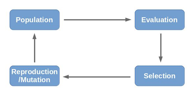
Process
Describing the process of an evolutionary algorithm is fairly simple with the above information. (1) First of all, a random population is generated. The individuals are evaluated (2) using the fitness function. With the known fitness values, a selection (3) of the population is drawn, so that the new population consists of adaptations of the fittest individuals of the previous population. The selection is then mixed up, mutated and allowed to generate offspring (4) resulting in the new population (1). This process is repeated until convergance or time runs out.
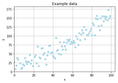
Example problem
To stress out the simplicity of an evolutionary optimization I want to fit a curve from data with random noise. The data is generated according to the formula
where \(R_{x}\) denotes a random, rational value drawn from a normal distribution with \(\mu = 0\) and \(\sigma = 15\).
import numpy as np

x = np.arange(0, 100)
y = 1.5 * x + np.random.normal(scale=15, size=100)
Individual
First of all we need a prototype for an individual. For the sake of convenience, I will start with an individual representing a linear function in the form
where \(a\) and \(b\) represent properties of the solution candidate, which can be mutated in the evolution process.
class LinearFunction(object):

    def __init__(self, a=0, b=0):
        self.a = a
        self.b = b

    def __call__(self, x):
        return self.a + self.b * x


def mutate(population):
    for linear_function in population:
        if random.random() < .5:
            linear_function.a += random.random() - .5
        else:
            linear_function.b += random.random() - .5
The mutate method iterates over the whole population, slightly changing a or b according to a random value between -0.5 and +0.5.
Fitness function
As a measurement of fitness, I'll base upon the simple RMSE metric. Since a higher RMSE-value means higher error whereas a higher fitness value means a fitter individual, I'll negate the RMSE-value to gain a proper fitness value.
def negative_rmse(linear_function):
    global x, y
    prediction = linear_function(x)
    error = prediction - y
    rse = np.sqrt(error ** 2)
    # ignore infinite values
    rse = np.ma.masked_invalid(rse)
    rmse = rse.mean()

    if np.isnan(rmse):
        rmse = np.inf

    return -rmse
Result
After running the simulation for 20 generations with a population size of 100 individuals per generation, I got to the result
which is a pretty fair guess of the original relationship of \(f(x) = 1.5 * x\).
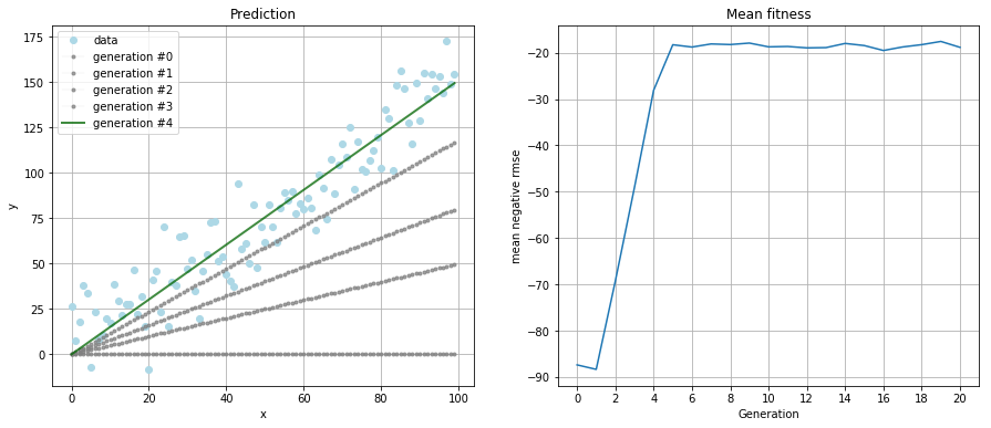
The left plot shows how the best individual of each generation performs on the data. The right plot is the mean fitness of the population in each generation. Also notice the convergence of the algorithm after five generations.
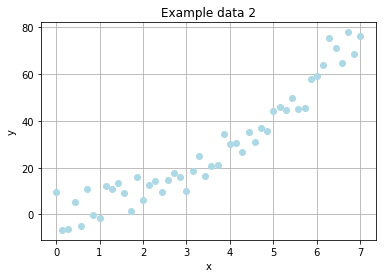
Example problem (sequel)
We've learned, that a simple linear function is way too easy for our simulated evolution. So how it will perform on non-linear data?
The new noised data will be expressed by
where \(R_x\) denotes a random, rational value drawn from a normal distribution with \(\mu = 0\) and \(\sigma = 5\).
x = np.linspace(0, 7)
y = .7 * x + 1.5 * x**2 + np.random.normal(scale=5, size=len(x))
Changes
In order to face the new problem, some changes have to be made:
- adapt individual to represent a polynomial
- modify the mutation to work with the new individual representation
The negative RMSE should still be suitable as fitness function.
Adapt Individual
The new individual should consist of multiple terms \(t \in T\), each in the form of \(t(x) = {f} * x^{p}\), where f and p are properties of the term. The final prediction of the individual is the sum of all its terms:
The split into multiple terms allows the mutation step to add or remove terms, resulting in a polynomial of undefined order. The polynomial can mutate according to the input data without the need to define the desired form in advance.
class Term(object):

    def __init__(self, factor, power):
        self.factor = factor
        self.power = power


class Polynomial(object):

    def __init__(self, terms):
        self.terms = terms

    def __call__(self, x):
        return sum(
            term.factor * (x ** term.power)
            for term
            in self.terms
        )

    def cleanup(self):
        powers = [term.power for term in self.terms]
        max_power = max(powers)
        min_power = min(powers)
        new_terms = []

        for power in range(min_power, max_power+1):
            factor = sum([term.factor for term in self.terms if term.power == power])
            new_term = Term(factor, power)
            new_terms.append(new_term)

        self.terms = new_terms

    def __repr__(self):
        return " + ".join([
            "{:.2f} * x^{:d}".format(term.factor, term.power)
            for term
            in self.terms
        ])
The cleanup method is just a helper to reduce a polynomial to one term per order.
Modified mutations
Instead of only modifying the parameters of a single term, we introduce two additional mutations adding or removing a term to/from an individual.
from copy import copy

def mutate_term(population):
    """Change `factor` or `power` of a term"""
    for polynomial in population:
        term = random.choice(polynomial.terms)

        if random.random() < .5:
            term.factor += random.random() - .5
        else:
            term.power += random.randint(-1, 1)

def add_term(population):
    """Copy random term"""
    for polynomial in population:
        term = random.choice(polynomial.terms)
        term = copy(term)
        polynomial.terms.append(term)

def remove_term(population):
    """Remove random term"""
    for polynomial in population:
        if len(polynomial.terms) <= 1:
            continue

        term = random.choice(polynomial.terms)
        polynomial.terms.remove(term)
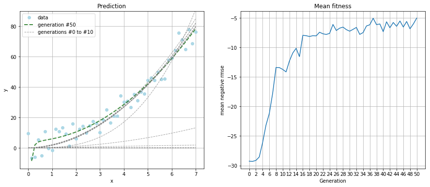
Result
Due to the increased complexity, I ran the simulation for 50 generations and kept the population size at 100.
The resulting polynomial was:
That's not as good a guess as the linear function from the first example. But a look at the prediction plot tells us the guess is still a good fit.
Conclusion
Evolutionary algorithms can definitely be used for curve fitting on linear and non-linear data. The whole process of optimization, mutation as well as the result can be easily understood, which is a huge benefit as opposed to using neural networks.
Since we can define individuals and mutations on our own, we are able to optimize the algorithm very well to a new problem, using our own ideas.
I can imagine great progress being made on evolutionary algorithms in the future and maybe even tackling domains, that today are reserved for deep neural networks and friends, since those are so appealingly simple.